Simulating Autonomous Robot Navigation with Python

Updated: Jul 29
Introduction
Autonomous mobile robots are becoming an increasingly common part of warehouse operations. They can transport inventory, support order picking, deliver materials to workstations, and reduce the amount of time employees spend walking through a facility.
Although their movement may appear simple, autonomous navigation requires several technologies to work together. A robot must observe its surroundings, distinguish open space from obstacles, determine where it needs to go, and calculate a safe route to reach its destination.
To explore this process, I developed a Python simulation that demonstrates how an autonomous robot can use LIDAR, occupancy-grid mapping, frontier detection, and path planning to explore an unknown environment.
The simulation provides a simplified view of how sensing, mapping, and decision-making come together in an autonomous system.
How Does LIDAR Work?
LIDAR, or Light Detection and Ranging, is a sensing technology commonly used by autonomous vehicles and mobile robots to measure the distance between the sensor and surrounding objects.
A LIDAR sensor emits a series of laser pulses and measures how long each pulse takes to return after striking an object. Because the speed of light is known, the sensor can use the pulse’s travel time to estimate the distance to a wall, rack, pallet, person, or other obstacle.
The basic calculation is:
Distance = Speed of Light × Travel Time ÷ 2
The calculation is divided by two because the laser pulse travels from the sensor to the object and then returns to the sensor.
A rotating LIDAR sensor performs this measurement across many angles. As the sensor sweeps around the robot, it produces a collection of distance readings that represent the surrounding environment.
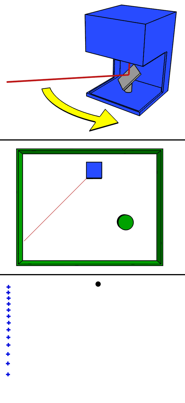
The first portion of the simulation visualizes this process. Laser beams extend outward from the robot until they encounter an obstacle, providing the measurements needed to begin constructing a map.
Building an Occupancy Grid
Individual LIDAR readings tell the robot where an obstacle was detected, but they do not automatically create a usable map.
To organize this information, the simulation divides the environment into a grid. Each cell in the grid represents a small section of physical space and is classified as one of three states:
Free space: The robot has observed the area and believes it can travel through it.
Occupied space: The robot believes the cell contains a wall or obstacle.
Unknown space: The robot has not yet observed the area.
This representation is known as an occupancy grid.
The simulation uses a log-odds occupancy grid, which allows the robot to represent uncertainty rather than treating every sensor measurement as completely accurate. Each observation increases or decreases the robot’s confidence that a grid cell is occupied.
For example, if multiple laser scans repeatedly detect an obstacle in the same location, the probability that the cell is occupied increases. If laser beams consistently pass through a cell without detecting anything, the robot becomes more confident that the space is open.
This allows the map to become progressively more accurate as the robot gathers additional information.
Exploring an Unknown Environment
Once the robot begins building a map, it must determine where to travel next.
In a known warehouse, a robot may already have a map of the building and receive a specific destination from a warehouse execution system. In an unknown environment, however, the robot must first explore the space and determine what is accessible.
The simulation uses a method known as frontier-based exploration.
A frontier is the boundary between known free space and unknown space. These locations are valuable because reaching them will allow the robot to observe additional parts of the environment.
The exploration process can be summarized as follows:
Scan the surrounding environment.
Update the occupancy grid.
Identify the boundaries between known and unknown space.
Select an accessible frontier.
Plan a route to that frontier.
Move toward the destination and repeat the process.
Rather than moving randomly, the robot selects destinations that progressively expand its knowledge of the environment.
Simulating a Limited Field of View
In the exploration simulation, the robot has a 90-degree field of view.
This means it can only observe a portion of its surroundings at any given time. Areas behind or beside the robot may remain unknown until it changes position or orientation.
Limiting the field of view makes the exploration problem more challenging and provides a clearer demonstration of how the robot builds its map incrementally.
As the robot moves, it discovers new corridors, obstacles, and open areas. Each observation changes the information available to the navigation system, potentially creating new exploration targets or invalidating an existing route.
This is an important characteristic of autonomous systems. The robot does not make one decision using a complete and permanent understanding of its environment. It continually updates its understanding and adjusts its decisions as new information becomes available.
Planning a Path with A*
After selecting a frontier, the robot must find a safe route to reach it.
The simulation uses the A* path-planning algorithm. A* searches through possible routes and evaluates each option based on:
The known cost of traveling from the robot’s current position.
The estimated remaining cost of reaching the destination.
The evaluation is commonly represented as:
f(n) = g(n) + h(n)
Where:
g(n) represents the cost of traveling from the starting position to the current point.
h(n) represents the estimated cost from the current point to the destination.
f(n) represents the estimated total cost of the route.
By considering both the travel already required and the estimated distance remaining, A* can efficiently identify a relatively short route through the known free space.
In this simulation, travel cost is primarily based on distance. A warehouse navigation system could incorporate additional factors, such as:
One-way aisles
Restricted areas
Congested intersections
Robot turning requirements
Pedestrian traffic
Different travel speeds
Temporary aisle closures
The shortest physical path is not always the best operational path. Route planning should represent the conditions and constraints that materially affect robot movement.
Updating the Route
A planned route is based on what the robot currently knows.
As the robot travels, its LIDAR sensor continues gathering information. A space that previously appeared open may contain an obstacle that was outside the robot’s field of view. A newly observed area may also provide a shorter or more accessible route.
When the occupancy grid changes, the robot evaluates whether its existing route is still valid. If the path is blocked, it uses A* to calculate a new route.
The overall navigation process becomes a repeating cycle:
Sense → Map → Plan → Move → Update
This feedback loop allows the robot to respond to changing information instead of following a fixed path regardless of what it encounters.
Applications in Warehouse Robotics

The simulation is a simplified representation of the navigation systems used by autonomous mobile robots in warehouses.
A production robot must account for considerably more complexity, including moving people, forklifts, pallets, other robots, sensor noise, localization error, vehicle dimensions, acceleration, braking, and safety requirements.
A complete warehouse robotics system may also need to coordinate hundreds of missions across an entire fleet. This introduces a second level of decision-making beyond the movement of an individual robot.
Fleet-level considerations may include:
Assigning robots to tasks
Managing traffic at intersections
Preventing aisle congestion
Coordinating workstation arrivals
Managing battery charging
Prioritizing urgent work
Recovering from blocked routes or equipment faults
An individually efficient route may not produce the best result for the complete system. For example, sending every robot along the shortest available route could create congestion and increase total mission time.
For that reason, autonomous robot design requires both local decision-making and system-level coordination.
Building on the Simulation
Several additional features could make the simulation more representative of a real warehouse robotics application.
Dynamic obstacles could be introduced to represent employees, forklifts, or other robots moving through the environment. Sensor noise could be added to demonstrate how uncertainty affects mapping accuracy. Alternative frontier-selection methods could compare the value of exploring nearby areas against the amount of new space likely to be discovered.
The simulation could also be expanded to include multiple robots. Each robot could share map information, coordinate exploration targets, and avoid creating traffic conflicts.
At the warehouse-system level, the navigation model could be combined with order data, task assignment, charging behavior, and workstation demand to evaluate how robot-level decisions affect throughput and labor productivity.
Conclusion
Autonomous navigation is not a single algorithm. It is a continuous process that brings together sensing, mapping, exploration, optimization, and control.
The robot must convert incomplete sensor measurements into an understanding of its surroundings, determine where it should move, calculate a route, and update that decision as new information becomes available.
Simplified simulations make these interactions easier to observe. They provide a useful environment for understanding the underlying technology, testing alternative strategies, and identifying the assumptions that influence system performance.
For warehouse automation, this type of analysis can help connect the behavior of an individual robot to the broader operational questions that ultimately determine whether a solution is safe, reliable, and effective.

Comments